I took a spatial analysis class last semester, and learned some pretty interesting things. As an all-time basketball fan, I decided to do some spatial analysis on Chris Paul’s jump shoot as my final project for that class. Here is a summary of the report. The only reason I chose Chris Paul is because he is my wife’s favorite player.

Introduction

The purpose of this project is to apply spatial analysis methods and procedures to the shooting data of a chosen basketball player. Chris Paul is the leading point guard in the NBA league today. He is famous for his sharp view on open opportunities on the court and deadly stable mid-range shooting (jumpshots taken in between the 3 point line and the painted area) over defense. I would like to answer two questions: first, does Chris Paul has a preference on where to make a shot; and second, is there a place on the court where Chris Paul is “unstoppable”.

Methods

The shooting log of Chris Paul from the 2014-2015 NBA season was scraped and downloaded from the http://stats.nba.com/ website with the help from this post. It contained detailed information regarding every shot the player made or missed at each game, such as the coordinates of the shot, the closest defender, the result of the shot (made/missed). Using the hoop as the reference point, the Y coordinate was the distance to the baseline, and X=0 was the line perpendicular to the baseline, crossing the hoop. Y can be negative since the hoop was within the court parameters, and a shot could be made behind the basket. The value of X coordinate was therefore the distance to the line X=0. Facing the basket, X was negative when the shoot was on the left side of the court, and it was positive when the shot was on the right side. Free throws were not included in the analysis, so only field goals were accounted for. Two pointers (a shot worth 2 points when made) could be distinguished from three pointers by their distance to the hoop, and coordinates of the shots.

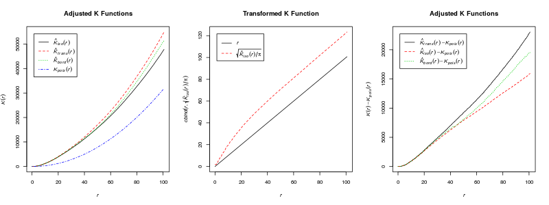
The shooting data was first mapped to a figure of basketball court using code from here . Without differentiating the made and missed shot, the complete spatial randomness was tested under the assumption of homogeneous Poisson processes using all shooting points. The Ripley’s K function was calculated and plotted, along with adjusted K function curves. We would like to know whether the distribution of the shoots on the court was homogeneous, and the result could tell us whether the player had a preference on where to shoot the ball on the court over the season.

One question that is of particular interest is whether the player had a higher percentage of making the shot rather than missing it at some regions on the court. To assess if the made shots are spatially aggregated, we need to compare their spatial distribution with the spatial distribution of the missed ones. One way to do this is to compare the intensity of the made and missed shots by the comparison of their K functions. The method was proposed by Rowlingson and Diggle and it was implemented in the Splancs library of R. Similar analytical approach was conducted in the Ramis et al. paper, studying the spatial distribution of childhood cancer. An interesting analogy can be found among several key parameters between the Ramis study and this project: population vs. total shots, cancer cases vs. shots made, and controls vs. shots missed.

A simulation was performed in the end to see what the goal percentage (number of shots made/total number of shots) should be when a significant difference can be detected. Given the same amount of shots and identical location, each shot was randomly assigned as made or missed following a predefined probability distribution. The K functions from simulated made and missed shots were compared and plotted.

Results and Discussion

Chris Paul attempted 1109 shots in the 2014-2015 season, made 541 and missed 569. Of the 1109 shots, 782 were two pointers, including 483 mid-ranges, and the rest 327 were three pointers.

Figure 1 Shotchart of Chris Paul Field Goal Attempts During 2014-2015 Regular Season

Figure 1 shown above is the shot chart summarizing all the shots attempted by Chris Paul last year. The green dots were shots made and red shows the ones missed. We can see that there were more attempted shots on the right side of the court. The shots were clustered under the hoop, and at the left corner. There was a clear gap between the three pointers and the mid-range shots.

The K function was constructed and plotted above without differentiating the made and missed shots. The distance is in 1/10 ft per unit as the width of a standard NBA court is 50 ft. The K function curve lies well above the range defined by the upper- and lower-envelope function, indicating a strong deviation from the complete spatial randomness. This is confirmed by the adjusted K functions shown above since the adjusted K curves are far from the K curve under theoretical Poisson distribution.

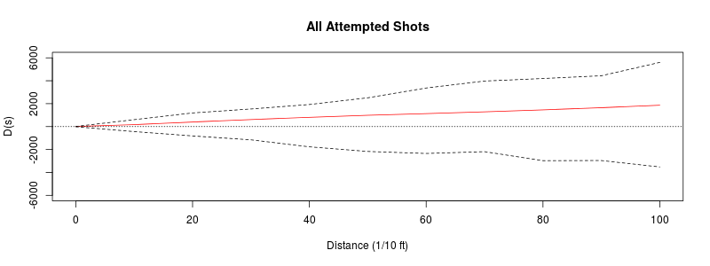
In order to compare the spatial distribution between made and missed shots, the difference between their K functions were (D) plotted above. The red line is the observed D, while the upper and lower theoretical bound were presented in dotted lines. Since the red line is within the envelope formed by the upper and lower bound, we conclude that the spatial distributions of made and missed shots are not significantly different. In other words, there were no areas on the court where Chris Paul shot better or worse than the rest. We can also perform similar analysis stratified by shooting zone, such as beyond 3 point arc, mid-range, in the paint, and within the restricted area, and the plots for stratified regions are shown on the last page. Those plots confirm that there are no regions where Chris Paul shot particularly better or worse since the red line is always within the envelope created by the upper and lower boundaries.

Conclusions

It is clear from the shot chart and the K function plot of all shot attempts that Chris Paul had a certain preference on where he would make shots. There were, however, no significant difference on the field goal success rate over various regions on the court. The field goal percentage for a decent NBA player is around 40%, which gives a made vs. missed ratio about 2:3. This ratio may not be large enough to detect for the proposed method. In order to determine when a difference in made and missed shots can be found, simulated tests were conducted. Given the same position and number of shots made by Chris Paul, simulated made/missed status was assigned to each attempt based on a predefined probability. We can see from the plots shown below that only when the field goal percentage is over 99%, can current method detect a significant difference. Some NBA players at center or power forward position would only attempt shots at very close range by dunking. They may have the highest field goal percentage, which is around 75%, but still not high enough to be considered significantly different between made and missed. Besides, these players of high field goal percentage tend to make their attempts under the basket, so all the shots are overlapped or tightly clustered, leaving no points for conducting the analysis.

It is therefore reasonable to say that the method proposed by Ramis et al for the analysis of cancer case distributions, regardless the close analogy between their examples and our situation, may not be applicable to our basketball shooting data. This is due to the fact that the field goal percentage of an average basketball player is usually close to 50%. We may have to try other methods to compare the spatial distributions in made and missed shots. Another possible approach is to treat the shooting as geostatistical data, and each point has a value of either 0 (missed) or 1 (made). We can build prediction models using krigging to estimate the propensity of making shots at a given location on the courts. There are several concerns using the methods. For example, there is a reference point on the court, which is the basket. According to the basketball common sense, the closer to the basket, the easier the shot is. This heterogeneity may not be well represented in the statistical model. This approach remains unexplored, awaiting for future pursuit.

References

Ramis R, Gómez-Barroso D, Tamayo I, García-Pérez J, Morales A, et al. (2015) Spatial Analysis of Childhood Cancer: A Case/Control Study. PLoS ONE10(5): e0127273.
Rowlingson BS, Diggle PJ. Splancs: spatial point pattern analysis code in S-Plus. Comput Geosci. 1993; 19: 627–655.